


■ Wilk's Lambda
1. Wilk's Lambda 란[1]
검증 통계치(test statistics)에서 많이 사용되는 검정 통계량
Wilks lambda ranges from 0 – 1 and the lower the Wilks lambda, the larger the between group
dispersion. A small (close to 0) value of Wilks' lambda means that the groups are well separated. A large (close to 1) value of Wilks' lambda means that the groups are poorly separated.
- 0 ~ 1 사이의 값을 가짐
- 1에 가까우면 그룹들이 잘 분류되지 않음
- 0에 가까우면 그룹들이 잘 분류됨
2. Wilk's Lambda 식 (Λ)

2.1 각 수식에 대한 개념
W: Within-groups sum of squares and cross-products matrix :: 그룹 내 제곱합과 대칭 행렬[2]
--> 클래스 내 분산과 같음
B: Between-groups sum of squares and cross-products matrix
--> 클래스 간 분산과 같음
T: Total sum of squares and cross-products matrix
[note] the cross product matrix X' X is a symmetric matrix.
- 2 참조 사이트에 가면 sum of square 에 대한 개념과 cross-product matrix에 대한 개념을 이해할 수 있음
2.2 각 요소에 대한 개념
g: is the number of group(그룹(클래스)의 수)
ni: is the number of observations in the ith group(i 번재 그룹에 속하는 패턴들의 수)
/Xi: The mean vector of the ith group(i 번째 그룹의 평균)
/X: The mean vector of the all the observations(전체 평균)
Xij: The jth multivariate observation in the ith group(i 번째 그룹에서 j 번째 나타난 다변량 관측 값; i행에 j번째 값)
2.3 수식 설명

그림에서 볼 수 있듯이 클래스간 분산(B)를 분모로 넣고 클래스내 분산(W)를 분자로 나누었을 경우 생각해 보면
- 클래스 내 분산이 작고, 클래스간 분산이 크면: 분류 하기 쉬움(결과 값이 작아짐)
- 클래스 내 분산이 크고, 클래스간 분산이 작으면: 분류 하기 어려움(결과 값이 커짐)
즉, Wilk's Lambda 수식에서 Lambda(Λ)의 값이 작을 수록 판별하기 수월한 능력을 가진다라고 이야기 할 수 있음.
3. 예제
레퍼런스 2번에 있는 값들을 사용하여 계산해 보자. 초점은 어떻게 Wilk's Lambda를 계산하는가 이다.
Formulation I |
Formulation II |
Formulation III |
|||
Cmax(X1) |
AUC(X2) |
Cmax(X1) |
AUC(X2) |
Cmax(X1) |
AUC(X2) |
0.342 |
2.1 |
0.169 |
1.097 |
0.091 |
0.724 |
0.11 |
0.747 |
0.295 |
1.76 |
0.264 |
1.538 |
0.279 |
1.833 |
0.381 |
2.294 |
0.463 |
2.417 |
0.2 |
1.32 |
0.173 |
1.024 |
0.19 |
1.379 |
0.207 |
1.245 |
0.37 |
2.384 |
0.101 |
0.737 |
step 1: 먼저 아래와 같이 다시 메트릭스를 구성하자.(보기 편하게)
Group |
Cmax(X1) |
AUC(X2) |
0.342 |
2.1 |
|
0.11 |
0.747 |
|
Formulation1 |
0.279 |
1.833 |
0.2 |
1.32 |
|
0.207 |
1.245 |
|
0.169 |
1.097 |
|
0.295 |
1.76 |
|
Formulation2 |
0.381 |
2.294 |
0.173 |
1.024 |
|
0.37 |
2.384 |
|
0.091 |
0.724 |
|
0.264 |
1.538 |
|
Formulation3 |
0.463 |
2.417 |
0.19 |
1.379 |
|
0.101 |
0.737 |
step 2: 관련 변수 값 구하기
A) 평균
Group |
Cmax(X1) |
AUC(X2) |
Formuldation1 |
0.2276 |
1.449 |
Formuldation2 | 0.2776 | 1.7118 |
Formuldation3 | 0.2218 | 1.359 |
B) 전체 평균
|
Cmax(X1) |
AUC(X2) |
| Total Mean | 2.242333 |
1.5066 |
Step 3: T 값 구하기
A) 각 raw 데이터에 컬럼 전체 평균을 빼줌( raw data - mean of each column)
Cmax(X1) | AUC(X2) |
0.099667 |
0.5934 |
-0.13233 |
-0.7596 |
0.036667 |
0.3264 |
-0.04233 |
-0.1866 |
-0.03533 |
-0.2616 |
-0.07333 |
-0.4096 |
0.052667 |
0.2534 |
0.138667 |
0.7874 |
-0.06933 |
-0.4826 |
0.127667 |
0.8774 |
-0.15133 |
-0.7826 |
0.021667 |
0.0314 |
0.220667 |
0.9104 |
-0.05233 |
-0.1276 |
-0.14133 |
-0.7696 |
- 이름을 Tmatrix 라고 임의로 지정
B) T 값 구하기: Tmatrix' * Tmatrix
여기서 '는 전치행렬(transposed matrix)
수행결과: T=
0.1751 |
0.9223 |
0.9223 |
5.0445 |
Step 4: W 값 구하기
A) 각 그룹별로 그룹 평균 빼기
Cmax(X1) |
AUC(X2) |
0.1144 |
0.651 |
-0.1176 |
-0.702 |
0.0514 |
0.384 |
-0.0276 |
-0.129 |
-0.0206 |
-0.204 |
-0.1086 |
-0.6148 |
0.0174 |
0.0482 |
0.1034 |
0.5822 |
-0.1046 |
-0.6878 |
0.0924 |
0.6722 |
-0.1308 |
-0.635 |
0.0422 |
0.179 |
0.2412 |
1.058 |
-0.0318 |
0.02 |
-0.1208 |
-0.622 |
B) 각 그룹별(클래스내) 분산 구하기
CovG1 = Formuldation1' * Formuldation1
CovG2 = Formuldation2' * Formuldation2
CovG3 = Formuldation3' * Formuldation3
covG1 =
0.0307 0.1845
0.1845 1.1223
covG2 =
0.0423 0.2619
0.2619 1.6442
covG3 =
0.0927 0.4203
0.4203 1.9419
C) 각 그룹 분산 더하기 최종 W 계산
covTotal =
0.1657 0.8667
0.8667 4.7084
Step 4: Wilk's Lambda 계산
Λ = |W|/|T|
W = 0.029
T = 0.033
Λ = 0.029/0.033 = 0.879
이상. Wilk's Lambda 의 값이 1의 값에 근접하고 있다. 때문에 Cmax와 AUC를 통해 뚜렷하게 목표로하는 대상을 구분하기 어렵다.
:: 오랜만에 쓰는군... 역시나 쉽지 않아.
4. 구현 결과

Reference
[1] http://www.ijpsi.org/VOl(2)1/Version_3/G0213644.pdf
[2] http://stattrek.com/matrix-algebra/sums-of-squares.aspx
'PatternRecognition' 카테고리의 다른 글
| Linear Discriminant Analysis(LDA) - C-Classes (0) | 2014.06.02 |
|---|---|
| Linear Discriminant Analysis(LDA) - 2 classes (0) | 2014.05.30 |
| Neural Networks: Data normalization (0) | 2014.04.25 |
| The Basic Artificial Neuron: Bias neuron(Backpropagation) (3) | 2014.04.23 |
| 기초 통계(Statistic) (0) | 2014.04.14 |
■ Linear Discriminant Analysis(LDA) - C-Classes
이전 글을 두개의 클래스를 판별하는 LDA에 대해서 알아 봤다. 그럼 여러개(C개)의 클래스를 어떻게 판별할 수 있을까? 접근은 2개의 클래스 판별 LDA 방법과 유사하다.
n-feature vectors를 가졌다면 다음과 같이 표현할 수 있다.

여기서 Y는 출력벡터, X는 입력벡터, W는 변환행렬이다.
- 즉 mxn입력 백터에 C개의 클래스를 LDA 분석을 하면 출력벡터는 c-1 by n개의 배열이 된다. 이에 중요한점은 각 클래스 마다 최적의 변환행렬을 계산해야 한다.
C개의 클래스를 가지는 입력 벡터를 LDA 분석하기 위한 단계는 다음과 같다.
1. 원래 데이터 차원에서 통계 계산
step 1: 클래스 내 분산 구하기


step 2: 클래스 간 분산 구하기


2. 투영된 데이터 차원에서 통계 계산
step 1: 평균 벡터 구하기

step 2: 클래스 내 분산 구하기

step 3: 클래스 간 분산 구하기

3. 목적행렬을 통한 최적 변환 행렬 찾기

- 최적 변환 행렬은 일반적인 고유값 문제 해결로 얻을 수 있는 최고 고유값에 해당하는 고유벡터가 됨
- C개의 클래스는 C-1개의 변환행렬을 가짐
4. 차원 축소

추가적으로 LDA 접근은 두 가지 방법으로 나뉘어짐
- 클래스 종속: 각 클래스 마다 변환행렬 생성
- 클래스 독립: 하나의 변환행렬 생성
5. 예제
LDA에 쓸 3개의 클래스 샘플 생성
1 2 3 4 5 6 7 8 9 10 11 12 13 14 15 16 17 18 19 20 21 22 23 24 25 26 27 28 29 30 31 32 33 34 35 36 37 38 39 40 41 42 43 44 45 46 47 48 49 50 51 52 53 54 55 56 57 58 59 60 61 62 63 64 65 66 67 68 69 70 71 72 73 74 75 76 77 78 79 80 81 82 | %clear clear %dataset Generation %let the center of all classes be Mu = [5;5]; %%for the first class Mu1=[Mu(1)-3; Mu(2)+7]; CovM1 = [5 -1; -3 3]; %%for the second class Mu2=[Mu(1)-2.5; Mu(2)-3.5]; CovM2 = [4 0; 0 4]; %%for the third class Mu3=[Mu(1)+7; Mu(2)+5]; CovM3 = [3.5 1; 3 2.5]; %generating feature vectors using Box-Muller approach %Generate a random variable following uniform(0,1) having two features and %1000 feature vectors U=rand(2,1000); %Extracting from the generated uniform random variable two independent %uniform random variables; u1 = U(:,1:2:end); u2 = U(:,2:2:end); %Using u1 and u2, we will use Box-Muller method to generate the feature %vectors to follow standard normal X=sqrt((-2).*log(u1)).*(cos(2*pi.*u2)); clear u1 u2 U; %now ... Manipulating the generated features N(0,1) to following certain %mean and covariance orher than the standard normal %First we will change its variance then we will change its mean %Getting the eigen vectors and values of the covariance matrix [V,D] = eig(CovM1); % D is the eigen values matrix and V is the eigen vectors matrix newX=X; for j=1:size(X,2) newX(:,j)=V*sqrt(D)*X(:,j); end %changing its mean newX=newX+repmat(Mu1, 1, size(newX,2)); %now our dataset for the first class matrix will be X1 = newX; %each column is a feature vector, each row is a single feature %...do the same for the other two classes with difference means and covariance matrices [V,D] = eig(CovM2); newX=X; for j=1:size(X,2) newX(:,j)=V*sqrt(D)*X(:,j); end newX=newX+repmat(Mu2, 1, size(newX,2)); X2 = newX; [V,D] = eig(CovM3); newX=X; for j=1:size(X,2) newX(:,j)=V*sqrt(D)*X(:,j); end newX=newX+repmat(Mu3, 1, size(newX,2)); X3 = newX; %draw 2d scatter plot figure; hold on; plot(X1(1,:), X1(2,:), 'ro', 'markersize',10, 'linewidth', 3); plot(X2(1,:), X2(2,:), 'go', 'markersize',10, 'linewidth', 3); plot(X3(1,:), X3(2,:), 'bo', 'markersize',10, 'linewidth', 3); |
위 코드 수행시 아래와 같이 출력됨

LDA matlab 코드는 다음과 같다.
1 2 3 4 5 6 7 8 9 10 11 12 13 14 15 16 17 18 19 20 21 22 23 24 25 26 27 28 29 30 31 32 33 34 35 36 37 38 39 40 41 42 43 44 45 46 47 48 49 50 51 52 53 54 55 56 57 58 59 60 61 62 63 64 65 66 67 68 69 70 71 72 73 74 75 76 77 78 79 80 81 82 83 84 85 86 87 88 89 90 91 92 93 94 95 96 97 98 99 100 101 102 103 104 105 106 107 108 109 110 111 112 113 | %% computing the LDA % class means Mu1= mean(X1')'; Mu3= mean(X2')'; Mu2= mean(X3')'; %overall mean Mu = (Mu1+Mu2+Mu3)./3; %class covariance matrices S1=cov(X1'); S2=cov(X2'); S3=cov(X3'); %within-class scatter matrix Sw=S1+S2+S3; %number of samples of each class N1=size(X1, 2); N2=size(X2, 2); N3=size(X3, 2); %between-class scatter matrix SB1=N1.*(Mu1-Mu)*(Mu1-Mu)'; SB2=N2.*(Mu2-Mu)*(Mu2-Mu)'; SB3=N3.*(Mu3-Mu)*(Mu3-Mu)'; SB=SB1+SB2+SB3; %computing the LDA projection invSw=inv(Sw); invSw_by_SB = invSw*SB; %getting the projection vectors %[V,D]=EIG(X) produces a diagonal matrix D of eigenvalues and a %full matrix V whose columns are the corresponding eigenvectors [V,D]=eig(invSw_by_SB); %the projcetion vectors - we will have at most C-1 projection vectors, %from which we can choose the most important ones ranked by their %corresponding eigen values ... lets investigate the two projection vectors W1=V(:,1); W2=V(:,2); %%lets visualize them... % we will plot the scatter plot to better visualize the features hfig=figure; axes1=axes('Parent',hfig,'FontWeight','bold','FontSize',12); hold('all'); %Create xLabel xlabel('X_1 - the first feature', 'FontWeight', 'bold', 'FontSize',12,'FontName', 'Garamond'); %Create yLabel ylabel('X_2 - the second feature', 'FontWeight', 'bold', 'FontSize',12,'FontName', 'Garamond'); %the fist class scatter(X1(1,:), X1(2,:),'r','LineWidth',2,'Parent',axes1); hold on %the second class scatter(X2(1,:), X2(2,:),'g','LineWidth',2,'Parent',axes1); hold on %the third class scatter(X3(1,:), X3(2,:),'b','LineWidth',2,'Parent',axes1); hold on %drawing the projection vectors %the first vector t=-10:25; line_x1 = t.*W1(1); line_y1 = t.*W1(1); %the second vector t=-5:20; line_x2 = t.*W2(1); line_y2 = t.*W2(2); plot(line_x1, line_y1, 'k-', 'LineWidth',3); hold on plot(line_x2, line_y2, 'm-', 'LineWidth',3); hold on %projection data samples along the projections axes %the first projection vector y1_w1 = W1'*X1; y2_w1 = W1'*X2; y3_w1 = W1'*X3; %projection limits minY=min([min(y1_w1), min(y2_w1), min(y3_w1)]); maxY=max([max(y1_w1), max(y2_w1), max(y3_w1)]); y_w1=minY:0.05:maxY; %for visualization lets compute the probability %density function of the classes after projection %the first class y1_w1_Mu = mean(y1_w1); y1_w1_sigma = std(y1_w1); y1_w1_pdf = mvnpdf(y1_w1',y1_w1_Mu,y1_w1_sigma); %the second class y2_w1_Mu = mean(y2_w1); y2_w1_sigma = std(y2_w1); y2_w1_pdf = mvnpdf(y1_w1',y2_w1_Mu,y2_w1_sigma); %the third class y3_w1_Mu = mean(y3_w1); y3_w1_sigma = std(y3_w1); y3_w1_pdf = mvnpdf(y1_w1',y3_w1_Mu,y3_w1_sigma); |

검은색이 고유값이 큰 고유벡터 값으로 판별되는 LD1 축이 되고, 다음 고유값에 따른 LD2 축이 보라색 선이 된다. 코드안에 차원축소를 한 데이터에 대해 PDF 분석 코드가 있다. 화면에 찍어야 하는데 그건 잘 모르겠다.
우선 LDA에 대해서 어떻게 접근해야 하는지 이제 좀 감이 잡힌다. 다시 LDA 전체 matlab 소스 코드를 첨부한다.
1 2 3 4 5 6 7 8 9 10 11 12 13 14 15 16 17 18 19 20 21 22 23 24 25 26 27 28 29 30 31 32 33 34 35 36 37 38 39 40 41 42 43 44 45 46 47 48 49 50 51 52 53 54 55 56 57 58 59 60 61 62 63 64 65 66 67 68 69 70 71 72 73 74 75 76 77 78 79 80 81 82 83 84 85 86 87 88 89 90 91 92 93 94 95 96 97 98 99 100 101 102 103 104 105 106 107 108 109 110 111 112 113 114 115 116 117 118 119 120 121 122 123 124 125 126 127 128 129 130 131 132 133 134 135 136 137 138 139 140 141 142 143 144 145 146 147 148 149 150 151 152 153 154 155 156 157 158 159 160 161 162 163 164 165 166 167 168 169 170 171 172 173 174 175 176 177 178 179 180 181 182 183 184 185 186 187 188 189 190 191 192 193 194 195 196 | %clear clear %dataset Generation %let the center of all classes be Mu = [5;5]; %%for the first class Mu1=[Mu(1)-3; Mu(2)+7]; CovM1 = [5 -1; -3 3]; %%for the second class Mu2=[Mu(1)-2.5; Mu(2)-3.5]; CovM2 = [4 0; 0 4]; %%for the third class Mu3=[Mu(1)+7; Mu(2)+5]; CovM3 = [3.5 1; 3 2.5]; %generating feature vectors using Box-Muller approach %Generate a random variable following uniform(0,1) having two features and %1000 feature vectors U=rand(2,1000); %Extracting from the generated uniform random variable two independent %uniform random variables; u1 = U(:,1:2:end); u2 = U(:,2:2:end); %Using u1 and u2, we will use Box-Muller method to generate the feature %vectors to follow standard normal X=sqrt((-2).*log(u1)).*(cos(2*pi.*u2)); clear u1 u2 U; %now ... Manipulating the generated features N(0,1) to following certain %mean and covariance orher than the standard normal %First we will change its variance then we will change its mean %Getting the eigen vectors and values of the covariance matrix [V,D] = eig(CovM1); % D is the eigen values matrix and V is the eigen vectors matrix newX=X; for j=1:size(X,2) newX(:,j)=V*sqrt(D)*X(:,j); end %changing its mean newX=newX+repmat(Mu1, 1, size(newX,2)); %now our dataset for the first class matrix will be X1 = newX; %each column is a feature vector, each row is a single feature %...do the same for the other two classes with difference means and covariance matrices [V,D] = eig(CovM2); newX=X; for j=1:size(X,2) newX(:,j)=V*sqrt(D)*X(:,j); end newX=newX+repmat(Mu2, 1, size(newX,2)); X2 = newX; [V,D] = eig(CovM3); newX=X; for j=1:size(X,2) newX(:,j)=V*sqrt(D)*X(:,j); end newX=newX+repmat(Mu3, 1, size(newX,2)); X3 = newX; %draw 2d scatter plot figure; hold on; plot(X1(1,:), X1(2,:), 'ro', 'markersize',10, 'linewidth', 3); plot(X2(1,:), X2(2,:), 'go', 'markersize',10, 'linewidth', 3); plot(X3(1,:), X3(2,:), 'bo', 'markersize',10, 'linewidth', 3); %% computing the LDA % class means Mu1= mean(X1')'; Mu3= mean(X2')'; Mu2= mean(X3')'; %overall mean Mu = (Mu1+Mu2+Mu3)./3; %class covariance matrices S1=cov(X1'); S2=cov(X2'); S3=cov(X3'); %within-class scatter matrix Sw=S1+S2+S3; %number of samples of each class N1=size(X1, 2); N2=size(X2, 2); N3=size(X3, 2); %between-class scatter matrix SB1=N1.*(Mu1-Mu)*(Mu1-Mu)'; SB2=N2.*(Mu2-Mu)*(Mu2-Mu)'; SB3=N3.*(Mu3-Mu)*(Mu3-Mu)'; SB=SB1+SB2+SB3; %computing the LDA projection invSw=inv(Sw); invSw_by_SB = invSw*SB; %getting the projection vectors %[V,D]=EIG(X) produces a diagonal matrix D of eigenvalues and a %full matrix V whose columns are the corresponding eigenvectors [V,D]=eig(invSw_by_SB); %the projcetion vectors - we will have at most C-1 projection vectors, %from which we can choose the most important ones ranked by their %corresponding eigen values ... lets investigate the two projection vectors W1=V(:,1); W2=V(:,2); %%lets visualize them... % we will plot the scatter plot to better visualize the features hfig=figure; axes1=axes('Parent',hfig,'FontWeight','bold','FontSize',12); hold('all'); %Create xLabel xlabel('X_1 - the first feature', 'FontWeight', 'bold', 'FontSize',12,'FontName', 'Garamond'); %Create yLabel ylabel('X_2 - the second feature', 'FontWeight', 'bold', 'FontSize',12,'FontName', 'Garamond'); %the fist class scatter(X1(1,:), X1(2,:),'r','LineWidth',2,'Parent',axes1); hold on %the second class scatter(X2(1,:), X2(2,:),'g','LineWidth',2,'Parent',axes1); hold on %the third class scatter(X3(1,:), X3(2,:),'b','LineWidth',2,'Parent',axes1); hold on %drawing the projection vectors %the first vector t=-10:25; line_x1 = t.*W1(1); line_y1 = t.*W1(1); %the second vector t=-5:20; line_x2 = t.*W2(1); line_y2 = t.*W2(2); plot(line_x1, line_y1, 'k-', 'LineWidth',3); hold on plot(line_x2, line_y2, 'm-', 'LineWidth',3); hold on %projection data samples along the projections axes %the first projection vector y1_w1 = W1'*X1; y2_w1 = W1'*X2; y3_w1 = W1'*X3; %projection limits minY=min([min(y1_w1), min(y2_w1), min(y3_w1)]); maxY=max([max(y1_w1), max(y2_w1), max(y3_w1)]); y_w1=minY:0.05:maxY; %for visualization lets compute the probability %density function of the classes after projection %the first class y1_w1_Mu = mean(y1_w1); y1_w1_sigma = std(y1_w1); y1_w1_pdf = mvnpdf(y1_w1',y1_w1_Mu,y1_w1_sigma); %the second class y2_w1_Mu = mean(y2_w1); y2_w1_sigma = std(y2_w1); y2_w1_pdf = mvnpdf(y1_w1',y2_w1_Mu,y2_w1_sigma); %the third class y3_w1_Mu = mean(y3_w1); y3_w1_sigma = std(y3_w1); y3_w1_pdf = mvnpdf(y1_w1',y3_w1_Mu,y3_w1_sigma); |
[1] http://www.di.univr.it/documenti/OccorrenzaIns/matdid/matdid437773.pdf
[2] http://www.bytefish.de/blog/pca_lda_with_gnu_octave/
'PatternRecognition' 카테고리의 다른 글
| Wilk's Lambda (2) | 2014.12.15 |
|---|---|
| Linear Discriminant Analysis(LDA) - 2 classes (0) | 2014.05.30 |
| Neural Networks: Data normalization (0) | 2014.04.25 |
| The Basic Artificial Neuron: Bias neuron(Backpropagation) (3) | 2014.04.23 |
| 기초 통계(Statistic) (0) | 2014.04.14 |
■ Linear Discriminant Analysis(LDA) - 2 classes
선형판별분석
1. 개념
- 클래스간 분산(between-class scatter)과 클래스내 분산(within-class scatter)의 비율을 최대화 하는 방식으로 특징벡터의 차원을 축소하는 기법
- 즉, 한 클래스 내에 분산을 좁게 그리고 여러 클래스간 분산은 크게 해서 그 비율을 크게 만들어 패턴을 축소하게 되면 잘 분류할 수 있겠구나!!
- LDA 판별에 있어서 아래 두 그림은 좋은 그리고 나쁜 클래스 분류에 대해 묘사하고 있다.

rate 값이 클수록 판별하기 좋은데 위 그림 중 왼쪽은 rate값이 크고 오른쪽 그림은 작다.
즉, rate 값이 클수록 판별하기 좋고, rate값이 작으면 판별하기 어렵다.
이렇게 rate값을 크게 만들기 위해 기준선을 잘 잡는게 중요하다. 다음 그림을 보며 이해하자.

위 그림에 보면 BAD 축을을 기준으로 1차원 매핑을 하게 되면 각 클래스를 판별하기 어렵다. 위에 rate 구하는 공식에 클래스간 분산과 클래스내 분산 비율이 작아진것이다. 반대로 GOOD 1차원 축을 보면 rate가 큰것을 예상할 수 있으며, 고로 판별하기 쉬울것이라는 생각이 든다.
====(2개의 클래스 LDA 분석)
2. LDA에서 차원 축소에 판별척도(잘 분류된 정도) 계산방법
LDA에서 좋은 판별 기준을 결정하기 위해 목적함수를 사용한다.(평가함수로도 불린다.)
- objective function = criterion function = 평가함수 / 목적함수
- 이러한 함수의 결과는 LDA 분류의 척도로써 사용된다.
두 가지 목적함수가 있다.
가. 일반적인 목적함수


위 척도 J(W)는 클래스간 분산을 고려하지 않고 평균만을 고려했기에 좋은 척도가 아니라고 한다.
이에 Fisher이라는 사람이 다음과 같은 함수를 만듬
나. Fisher's criterion function

여기서 


그림과 같이 글래스간 분산도 고려하여 평균차이에 대한 비율로 척도를 계산함
- 이 값이 크면 클수록 좋음

3. 최적 분류를 위한 변환행렬 찾기
그럼 최고 좋은 값을 가지는 즉, 분류를 가장 잘 할수 있는 변환행렬은 어떻게 구할까? 이에 Fisher 선생님이 다음과 같은 공식을 만들었다.
3.1 Fisher’s Linear Discriminant(1936)
최적의 변환 행렬
- 최적의 변환 행렬을 만들기 위해 Fisher's criterion function 을 미분하여 0의 값을 가지게 수식을 수정한 결과이다. 미분값이 0 이면 기울기가 0라는것이다. 즉 최고점(global maximum point)이라는 점!!
- 여기에 일반화된 고유값 문제 해결을 통해 최적의 변환행렬을 계산해냄

참고
argmax(p(x)) : p(x)를 최대가 되게하는 x 값
max(p(x)) p(x) 중 최대값
argmin(p(x)) : p(x)를 최소가 되게하는 x 값
min(p(x)) : p(x) 중 최소값
4. 2개의 클래스를 LDA 분석하기 - Matlab

step 2: 각 클래스 내 분산 계산

step 3: 클래스 간 분산 계산
step 4: 고유값 및 고유벡터 계산
- 최고의 고유값을 가지는 고유벡터와 원행렬을 곱하면 된다.
1 2 3 4 5 6 7 8 9 10 11 12 13 14 15 16 17 18 19 20 21 22 23 24 25 26 27 28 29 30 31 32 33 34 35 36 37 38 39 | X = [4 2;2 4;2 3;3 6;4 4;9 10;6 8;9 5;8 7;10 8]; %입력 데이터 c = [ 1; 1; 1; 1; 1; 2; 2; 2; 2; 2;]; %입력 데이터 그룹 분류 c1 = X(find(c==1),:) %클래스 1에 해당하는 입력 데이터 매핑 c2 = X(find(c==2),:) %클래스 2에 해당하는 입력 데이터 매핑 figure; %그림 그리자 hold on; %잡고 있으려므나~~ p1 = plot(c1(:,1), c1(:,2), 'ro', 'markersize',10, 'linewidth', 3); %클래스 1 좌표 찍으렴 p2 = plot(c2(:,1), c2(:,2), 'go', 'markersize',10, 'linewidth', 3) %클래스 2 좌표 찍으렴 xlim([0 11]) %그래프 x의 좌표를 범위를 0-11까지 늘리자 ylim([0 11]) %그래프 y의 좌표를 범위를 0-11까지 늘리자 classes = max(c) %클래스가 몇개인지 보자구웃 mu_total = mean(X) %전체 평균 계산 mu = [ mean(c1); mean(c2) ] %각 클래스 평균 계산 Sw = (X - mu(c,:))'*(X - mu(c,:)) %클래스 내 분산 계산 Sb = (ones(classes,1) * mu_total - mu)' * (ones(classes,1) * mu_total - mu) %클래스간 분산 계산 [V, D] = eig(Sw\Sb) %고유값(V) 및 고유벡터(D) % sort eigenvectors desc [D, i] = sort(diag(D), 'descend'); %고유값 정렬 V = V(:,i); % draw LD lines scale = 5 pc1 = line([mu_total(1) - scale * V(1,1) mu_total(1) + scale * V(1,1)], [mu_total(2) - scale * V(2,1) mu_total(2) + scale * V(2,1)]); set(pc1, 'color', [1 0 0], 'linestyle', '--')%가장 큰 고유값을 가지는 선형판별 축 그리자 scale = 5 pc2 = line([mu_total(1) - scale * V(1,2) mu_total(1) + scale * V(1,2)], [mu_total(2) - scale * V(2,2) mu_total(2) + scale * V(2,2)]); set(pc2, 'color', [0 1 0], 'linestyle', '--')%두번째 고유값을 가지는 선형판별 축 그리자 |
보면 빨강색 선이 가장 좋은 LD 축이 되고 녹색이 나쁜 LD 축이 된다.

그럼 가장 좋은 LD1축으로 투영을 시켜 보자 . 위 코드 상태에서 바로 아래와 같이 명령어를 입력하면 된다.
1 2 3 4 5 6 7 8 9 10 11 12 13 14 15 16 17 18 19 20 21 22 | %First shift the data to the new center Xm = bsxfun(@minus, X, mu_total) %원래 데이터 평균 빼기 %then calculate the projection and reconstruction: z = Xm*V(:,1) %차원 축소 % and reconstruct it p = z*V(:,1)' %LD 축에 데이터 맞추기 위해 재구성 p = bsxfun(@plus, p, mu_total) %재구성된 데이터 평균더하기 %plotting it: % delete old plots delete(p1);delete(p2); % 이전 그려진 plot 데이터 삭제 y1 = p(find(c==1),:) %클래스 1 데이터 y1에 입력 y2 = p(find(c==2),:)%클래스 2 데이터 y2에 입력 p1 = plot(y1(:,1),y1(:,2),'ro', 'markersize', 10, 'linewidth', 3); p2 = plot(y2(:,1), y2(:,2),'go', 'markersize', 10, 'linewidth', 3); %찍어라 얍얍 %result - 원래 1차원으로 축소한 결과 result0 = X*V(:,1); % PDF그리기 위해 ... result1 = X*V(:,2); |

위 예제는 2개의 클래스를 가지고 LDA 분석하는 방법들이다.
[1] http://www.di.univr.it/documenti/OccorrenzaIns/matdid/matdid437773.pdf
[2] http://www.bytefish.de/blog/pca_lda_with_gnu_octave/
'PatternRecognition' 카테고리의 다른 글
| Wilk's Lambda (2) | 2014.12.15 |
|---|---|
| Linear Discriminant Analysis(LDA) - C-Classes (0) | 2014.06.02 |
| Neural Networks: Data normalization (0) | 2014.04.25 |
| The Basic Artificial Neuron: Bias neuron(Backpropagation) (3) | 2014.04.23 |
| 기초 통계(Statistic) (0) | 2014.04.14 |
■ Neural Networks: Data normalization
http://www.cs.sunysb.edu/~cse634/ch6NN.pdf
뉴럴 네트워크에서는 입력과 출력 데이터의 정규화가 필요하다. 위 사이트에 보면 데이터 정규화 방법으로 두개가 나와 있다.
All values of attributes in the dataset has to be changed to contain values in the interval [0,1], or [-1,1].
모든 데이터는 0~1, -1~1 사이 값에 포함되도록 바꿔야 한다.
Two basic normalization techniques:
- Max-Min normalization
- Decimal Scaling normalization
Max-Min normalization formula

Example: We want to normalize data to range of the interval [0,1].
We put: new_max A=1, new_min A = 0
Say, max A was 100 and min A was 20(That means maximum and minimum values for the attribute A).
Now, if v=40(if for this particular pattern, attribute value is 40), v' will be calculated as,
v'=(40-20)*(1-0)/(100-20)+0
= (20 * 1)/80
= 0.4(?) 아닌거 같은데... 0.25 아닌가?!!
Decimal Scaling Normalization formula

where j is the smallest integer such that max|v’|<1.
Example :
A–values range from -986 to 917. Max |v| = 986.
v = -986 normalize to v’= -986/1000 = -0.986
'PatternRecognition' 카테고리의 다른 글
| Linear Discriminant Analysis(LDA) - C-Classes (0) | 2014.06.02 |
|---|---|
| Linear Discriminant Analysis(LDA) - 2 classes (0) | 2014.05.30 |
| The Basic Artificial Neuron: Bias neuron(Backpropagation) (3) | 2014.04.23 |
| 기초 통계(Statistic) (0) | 2014.04.14 |
| Principal Component Analysis(주성분 분석) (0) | 2014.04.12 |
■ The Basic Artificial Neuron: Bias neuron(Backpropagation)
역전파 알고리즘 - 바이어스 노드
역전파 알고리즘은 각 뉴런의 출력 신호를 결정하기 위해서 입력(입력 신호와 연결 무게를 곱하고 나서 모두 합한값)에 활성화 함수(Activation Function)를 적용한다.
- 활성화 함수의 임계값 변동을 흡수하기 위한 가중치를 바이어스(편견)이라고 하며, 항상 1의 값을 가진다.
여러 활성화 함수 그림이다.
여기서 질문이 생긴다. 활성화 함수의 임계값 변동을 흡수(?-책에서 이렇게 씀)하기 위한 가중치 바이어스 노드를 항상 1로 설정한다라고 되어 있는데 왜 1인가 그리고 구체적인 이유가 무엇인가?
우선 구글링 한 정보를 정리하면 다음과 같다.
http://stackoverflow.com/questions/2480650/role-of-bias-in-neural-networks
http://stackoverflow.com/questions/8039313/why-is-a-bias-neuron-necessary-for-a-backpropagating-neural-network-that-recogni
답변에 보면 바이어스 값(bias value)는 성공적인 학습을 위해 활성화 함수를 좌우로 움직일 수 있게 해준다라고 한다. 단순한 예제를 보면 다음과 같다.
Case 1 : 바이어스 없이 하나의 입력과 출력의 구성

출력은 입력 x와 가중치 w0의 곱을 활성화 함수에 넣어 계산할 수 있다.

위 그림은 활성화 함수를 sigmoid로 하고 가중치 w0의 값이 0.5, 1.0, 2.0으로 변화 할때 입력과 출력에 관한 결과 그래프 이다. 위 그래프에서 보면 가중치 값이 변화함에 따라 sigmoid 의 가파름(steepness) 정도가 변화는 것을 확인할 수 있다. 이 결과는 유용하지만 만약 입력이 2개이고 출력이 하나인 네트워크를 구성할때 변화하는 시그모이드 함수의 steepness는 동작하지 않는다고 한다. (먼 예기야?)
위 커브들을 오른쪽으로 모두 옴기길 원하면 바이어스를 사용해야 한다.
다음 case를 보고 차이점을 보자
Case2: Case1 + Bias Neuron

그림에 보면 입력층에 Bias Neuron을 추가된 것을 확인할 수 있다. 그럼 출력은 sig(w0*x+w1*1.0)으로 계산될 수 있다. 아래 그림은 w1의 변화에 따른 네트워크 출력에 대한 그래프이다. (w0 = 1.0)

그림에 보면 바이어스 뉴런을 하나 추가하여 가중치 w1의 변화에 따라 출력이 좌우로 움직이(shift)되는 것을 확인할 수 있다. 아하!!!(센스 있는 사람은 눈치 챘을 것이다.)
@user1621769: The main function of a bias is to provide every node with a trainable constant value (in addition to the normal inputs that the node recieves). You can achieve that with a single bias node with connections to N nodes, or with N bias nodes each with a single connection; the result should be the same. – Nate Kohl Mar 24 '13 at 13:24
위 빨간색을 보면 중요한 얘기를 하고 있다.
바이어스의 중요한 기능은 훈련 가능한 상수 값을 가지는 모든 노드를 제공하는 것이다.
즉 바이어스 노드 없이 훈련 가능한 것들도 있지만 아마 다른 경우에 sigmoid 임계 범위에 있지 않은 값들의 출력은 의미가 없어져 훈련이 되지 않을 수도 있다.
http://www.nnwj.de/backpropagation.html
위 사이트에서 보면 보다 이해하기 쉬울 것이다.
http://www.mathworks.co.kr/kr/help/nnet/ug/perceptron-neural-networks.html
여기 사이트에서도 bias 의 역할을 설명하고 있다. 바이어스의 또 다른 역할은 기본 영역에서 항상 시프트하여 경계를 결정하게 해 줌 아래와 같이 점선에서 실선으로 바이어스를 적용하여 경계를 옴김

그럼 실제 뉴럴 계층에 bias neuron을 어떻게 적용시켜야 하나 문제다. 다음 그림을 보자.
http://ufldl.stanford.edu/wiki/index.php/Neural_Networks
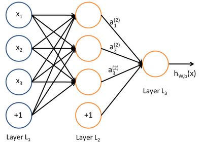
왼쪽 부터 입력 레이어(L1), 히든 레이어(L2), 출력 레이어(L3)로 나타난다. 보면 bias neuron이 입력과 히든레이어에 존재한다.
바이어스 뉴런은 다음 계층에 연결되지만 이전 계층에는 연결되지 않는 특징을 가진다.
입력층: 입력 노드(d) + 바이어스 노드(1)
은닉층: 은닉 노드(p) + 바이어스 노드(1)
은닉층의 노드 개수를 p라고 할때 하나의 바이어스 노드를 더해 은닉층의 총 노드 개수는 p+1개가 된다.
출력층: 원하는 출력 노드 수(m)
그럼 입력층과 은닉층 사이 가중치는 몇개?
입력층: d+1
은닉층: p
입력층과 은닉층의 가중치: (d+1)*p 개
그럼 은닉층과 출력층의 가중치는 몇개?
은닉층: p+1
출력층: m
은닉층과 출력층의 가중치: (p+1)*m 개
위 그림은 Basic Structure of an artificial neuron 그림이다. 맘에 들어서 가져 왔다. 자세한 설명은
http://engineeronadisk.com/book_modeling/neural.html
에 있다.
'PatternRecognition' 카테고리의 다른 글
| Linear Discriminant Analysis(LDA) - C-Classes (0) | 2014.06.02 |
|---|---|
| Linear Discriminant Analysis(LDA) - 2 classes (0) | 2014.05.30 |
| Neural Networks: Data normalization (0) | 2014.04.25 |
| 기초 통계(Statistic) (0) | 2014.04.14 |
| Principal Component Analysis(주성분 분석) (0) | 2014.04.12 |